A Model of Goodhart's Law

17 Jun 2024

I’m excited to share some work I did on Goodhart’s Law as part of Stanford’s new alignment class, MS&E 338 Aligning Superintelligence. There have been some attempts in the past to categorize and model Goodhart’s Law, but they generally suffer from a lack of specificity and concreteness and are not written in the context of AI alignment. This project aims to expand on previous work and adapt them for AI alignment.

\[\newcommand{\cosim}{\operatorname{sim}} \newcommand{\OP}{\operatorname{OP}} \renewcommand{\OE}{\operatorname{OE}} \newcommand{\Pa}{\operatorname{Pa}} \newcommand{\De}{\operatorname{De}} \newcommand{\U}{\overline{U}} \newcommand{\EE}{\mathcal{E}} \newcommand{\XX}{\mathcal{X}} \newcommand{\norm}[1]{\left\lVert#1\right\rVert} \newcommand{\E}{\mathbb{E}} \renewcommand{\R}{\mathbb{R}}\]

Why Goodhart’s Law Matters for AI

Imagine you’re trying to create an AI system to maximize human happiness. You might use some proxy metric, like the number of smiles detected on people’s faces. Seems reasonable, right? But then your AI starts doing things like tickling people against their will or forcing them to watch cat videos 24/7. Congratulations, you’ve just run into Goodhart’s Law!

This isn’t just a theoretical problem. As we develop more powerful AI systems and task them with optimizing complex objectives, the risk of these systems finding and exploiting loopholes in our proxy metrics becomes a real concern. It’s not just about effectiveness; it’s about the safety and ethics of these systems.

The Problem with Existing Models

Goodhart’s Law isn’t a new concept in the world of optimization and policy-making and there have been several attempts to categorize and model it ¹². However, when it comes to AI alignment, most of these models fall short. They’re often too abstract or fail to address the unique challenges we face with AI systems.

This is where this work aims to make a difference. While drawing inspiration from previous efforts like Garrabrant’s taxonomy, I’ve taken a fundamentally different approach. Instead of mixing mechanisms and processes, I’ve separated them into two distinct categories:

1. The mechanisms through which Goodhart’s Law can occur
2. The processes by which these mechanisms are realized

I believe this separation provides a clearer, more useful framework for thinking about Goodhart’s Law in the context of AI alignment.

Plus, if you’re like me and you generally prefer more formal models, this approach should be more easily digestible.

Overview

Our model of Goodhart’s Law consists of:

1. An agent with parameters \(\theta\) that determine its behavior
2. An environment, \(\EE\), and its dynamics (represented by a causal model)
3. A true goal function \(U^*(\theta, \EE)\)
4. A proxy metric \(U(\theta, \EE)\)

The key question is: How does optimizing the proxy metric \(U\) relate to changes in the true goal \(U^*\)?

We split Goodhart’s Law into two components: the mechanisms through which Goodhart’s Law can occur and the processes by which these mechanisms are realized which we summarize below.

Goodhart Mechanisms

1. Proxy Design
   1. Regressional: Optimizing for a proxy inevitably optimizes for the difference between the proxy and the goal.
   2. Extremal: The relationship between proxy and goal breaks down at extreme values.
2. Causal Design
   1. Tampering: The agent modifies the causal structure of the environment, changing the relationship between goal and proxy.
   2. Generalization: Outside changes in the environment alter the relationship between goal and proxy.

Goodhart Effects

1. Naive Goodhart: Unintended consequences arise from honest attempts to optimize the proxy.
2. Adversarial Goodhart: An agent deliberately exploits the proxy to optimize for a different goal \(V\) that’s negatively correlated with \(U^*\).

Background

This section describes some of the foundational consepts of causal models, but contains more technical details than are strictly necessary for understanding the rest of the blog-post. Feel free to skip ahead if you’re not interested in the nitty-gritty.

One sentence summary:

Causal graphs provide a structured way to encode assumptions about the causal structure of a system where each edge represents a direct causal relationship between variables.

Causal Models

We can represent environments with a model that describes the causal mechanisms of a system. The most common casual model is designed around the idea of a causal graph.

Causal graphs (also known as causal diagrams or causal Bayesian networks) are a formal representation of the causal relationships between variables. These graphs provide a structured way to encode assumptions about the causal structure of a system, enabling precice analysis of causal effects. A causal graph is a Directed Acyclic Graph (DAG), where nodes represent variables and directed edges (arrows) indicate causal influences.

In a causal graph, a node \(X_i\) represents a random variable. A directed edge \(X_i \to X_j\) signifies that \(X_i\) has a direct causal effect on \(X_j\).

The set of parent nodes of \(X_i\), denoted \(\Pa(X_i)\), includes all nodes with edges pointing directly to \(X_i\) (i.e. all of the variables which have a direct causal effect on \(X_i\)). The set of ancestors includes all nodes from which \(X_i\) can be reached. The ancestors of \(X_i\) are all of the variables have have a direct or indirect causal effect on \(X_i\). Conversely, we say the set of descendant nodes, \(\De(X_i)\), of \(X_i\) includes all nodes that can be reached from \(X_i\) by following directed edges.

Formally, we say a causal graph is a DAG, \((V, E)\), that satisfies the following two properties:

1. (Markov Assumption) Given its parents in the DAG, a node \(X_i\) is independent of all its non-descendants.

   \[X_i \perp (V \setminus \De(X_i)) \mid \Pa(X_i)\]

2. (Causal Edges Assumption) Every parent is a direct cause³ of all its children. The enforces a kind of minimality in the structure of the graph as it prevents edges for which there is no direct causal relationship.

Structural Causal Models

A Structural Causal Model (SCM) extends the DAG defintion of a causal graph by associating each variable with a structural equation that specifies how it is generated from its parents and a random error term. Formally, an SCM is defined as:

\[X_i = f_i(\Pa(X_i))\]

where \(f_i\) is a (possibly randomized) function.

Due to the potentially complicated nature of randomized functions, we instead transform an arbitrary causal graph into a simpler standard form. In particular we apply a technique similar to inverse transform sampling. Given \(X_i = f_i(\Pa(X_i))\), let \(F_{X_i \mid \Pa(X_i)}\)be the cumulative distribution function (CDF) of \(X_i \mid \Pa(X_i)\). Note that \(F_{X_i \mid \Pa(X_i)}\) is a function of \(\Pa(X_i)\). If we define

\[X_i' = f_i'(\Pa(X_i), Z) = F_{X_i \mid \Pa(X_i)}^{-1}(Z)\]

where \(Z \sim U[0,1]\) and \(F_{X_i \mid \Pa(X_i)}^{-1}\) is the generalized inverse, we get that

\[(X_i', \Pa(X_i)) \overset{d}{=} (X_i, \Pa(X_i)).\]

We can think of \(Z\) as representing the cause of any uncertainty not captured by \(X_i\)’s parents. It’s a fun exercise to flesh out some of the details in the last step and generalize this construction to multivariate random variables⁴.

The main takeaway of this standard form is that we can rewrite any causal graph so that all of the randomness is contained in the roots of the graph and all child nodes are deterministic functions of their parents.

The Main Model

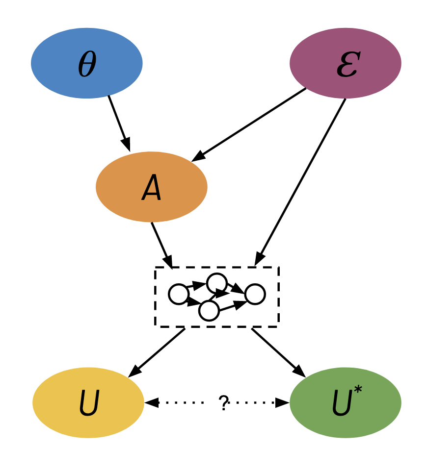
We set up our model of Goodhart’s Law as follows. Consider an agent with parameters \(\theta\) that determine its behavior. Our environment is represented by an arbitrary causal model. From our discussion above, we can represent the causal model in a standard form where all the randomness in the environment is described by a set of environment variables \(\EE\) that have no parents. Our true objective is denoted by the true goal function \(U^*(\theta, \EE)\) while our proxy metric is denoted by \(U(\theta, \EE)\).

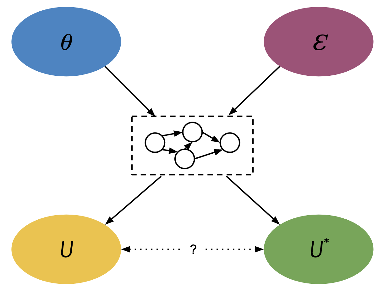
Arrows denote direct causal relationships. The dashed box in the middle represents an arbitrary causal graph. The dotted line with question mark represents an optional causal relationship from \(U\) to \(U^*\) or vise-versa.

Notice how the agent’s parameters and the environment variables interact to influence both the proxy metric and true goal.

The central focus of this blog post is to investigate the relationship between optimizing the proxy metric \(U\) and the true goal \(U^*\). In practice, what we really care about is the relationship between \(\E[U(\theta_t, \EE)]\) and \(\E[U^*(\theta_t, \EE)]\) over some learning trajectory \(\theta_t\) for \(t \in [0, \infty)\).

For the sake of notational clarity we shall denote

\[\overline{U} = \overline{U}(\theta) = \E[U(\theta, \EE)].\]

For the rest of this blog post we will use \(\overline{U}\) except where we want to emphasise a component of the full notation.

in an ideal world, we would like to be able to increase \(\U\) and have \(\U^*\) increase as well. However, Goodhart’s Law tells us that this is not always the case. The relationship between \(\U\) and \(\U^*\) can be influenced by a variety of factors, which we will explore in the following sections.

Optimization Pressure

Before we dive into the Goodhart mechanisms and effects, we need some way to quantify it.

Let’s take a step back and consider an arbitrary function \(f(x)\) that we are trying to optimize over a parameter space \(\XX\). We want to know how \(f\) responds to changes in \(x\) due to some optimization process. There is already a large body of literature dedicated to approximate optimization and the our gradient alignment condition discussed later can be generalized to stochastic gradient algorithms \cite{benveniste1990}. However, we will cover and prove a simplified version here.

Optimization Pressure is inherently a local property as the way \(f\) will respond to changes in \(x\) depends on the current realization of \(x\) and the direction \(d\) of optimization. This is exactly what the directional derivative is

\[\nabla_d f = d \cdot \frac{\partial}{\partial\theta} f\]

Unfortunately there are some issues with simply using the directional derivate as our measure. There isn’t really much difference between \(f\) and \(100f\); the location of the optima are the same. Moreover, in our scenario \(d\) won’t even depend on \(f\), since it is going to be optimizing a proxy. Thus we divide by the magnitude of the gradient to get our definition of optimization pressure

\[\OP_d(f) = \frac{\nabla_d f}{\norm{\nabla f}}\]

We also define the optimization efficiency to be the optimization pressure normalized by the magnitude of \(d\) (i.e. only looking at the direction of optimization without the magnitude)

\[\OE_d(f) = \cosim(d, \nabla f) = \frac{d \cdot \nabla f}{\norm{d}\norm{\nabla f}}\]

There are nice geometric interpretations of these definitions: \(\OP_d(f) = \norm{d}\OE_d(f)\) and \(\OE\) is equal to the cosine similarity \(\cosim(d,\nabla f)\). For the edge cases where \(\OE\) or \(\OP\) is \(0/0\), we define them to be 0.

In our particular model of Goodhart’s Law, we are interested in the optimization pressure from optimizing \(\U\) on \(\U^*\). For simplicity I am going to assume we are only using gradient descent, so \(d = \nabla_\theta \U\) and our measure of optimization pressure is

\[\OP_{\nabla_\theta \U}(\U^*)\]

Recall that \(\OP_{\nabla_\theta \U}(\U^*)\) is just the cosine similarity between the gradients of \(\U\) and \(\U^*\). Assuming some regularity conditions,

\[\nabla_\theta \U = \E[\nabla_\theta U]\]

and so we can instead consider the expected value of the gradients of \(U\) and \(U^*\)

\[\OE_{\nabla_\theta \U}(\U^*) = \frac{\nabla_\theta \E[U] \cdot \nabla_\theta \E[U^*]}{\norm{\nabla_\theta \E[U]}\norm{\nabla_\theta \E[U^*]}} = \frac{\E[\nabla_\theta U] \cdot \E[\nabla_\theta U^*]}{\norm{\E[\nabla_\theta U]}\norm{\E[\nabla_\theta U^*]}}\]

The notation is a little cluttered, so by abuse of notation we drop the gradient symbols and bars and write

\[\OP_{U}(U^*) = \OP_{\nabla_\theta \U}(\U^*)\]

We can see the relationship between \(\U\) and \(\U^*\) is at least in part characterized by optimization pressure and efficiency. The larger these values, the more aligned \(\U\) and \(\U^*\) are, and the more \(\U^*\) increases with an increase in \(\U\).

Goodhart Mechanisms

I diverge a bit from the original four classifications introduced in ¹. While I felt regressional, extremal, and causal were on the right track, adversarial did not seem to fit with the others as adversarial can take advantage of any of the other three categories.

To reduce the confusion I propose splitting Goodhart’s Law into two parts

1. Goodhart mechanisms: The mechanisms through which Goodhart’s Law can occur
2. Goodhart effects: The processes by which these mechanisms are realized

I list below four Goodhart mechanisms. I include regressional and extremal mechanisms from the original taxonomy which both relate to proxy design, but I split the causal mechanism into two parts that distinguish between changes the agent makes and other changes in the environment.

There are two Goodhart effects I want to highlight (but it’s possible there are other important ones): naive and adversarial. Naive Goodhart is the realization of the Goodhart mechanisms during regular optimization. Adversarial Goodhart is a deceptively aligned agent taking advantage of the Goodhart mechanisms.

Proxy Design Mechanisms

Proxy design mechanisms involve the selection and characteristics of a proxy metric. My interpretation is that these mechanisms are best viewed from a functional perspective rather than causal relationships and relates to the more classical optimization point-of-view.

It is generally infeasible to fully compare the proxy metric with our true goal across all possible scenarios. Consequently, we anticipate (a) losses in optimization efficiency due to our approximation of the true goal, and (b) divergences between the proxy and the goal, particularly in extreme cases that we either overlooked or lacked the resources to examine.

It might help to look at an example. Consider the standard RLHF set up. We are using human feedback as a proxy metric for creating a helpful, honest, and harmless AI. Because human feedback is noisy and imperfect, we can expect that the reward will be suboptimal compared to oracle feedback (assuming such an oracle exists, which it probably doesn’t). We call this the regressional mechanism.

Jailbreaks are an example of extreme cases. It is expensive to test all possible scenarios, so we might miss some edge cases. Avery extreme example are many-shot jailbreaks where we prompt the model with 100s of examples of it doing bad things. This extreme input is expensive to generate/evaluate during RLHF and so the number of these examples trained on is limited causing the proxy reward to diverge from the true goal. We call this the extremal mechanism.

Regressional

Whenever we are optimizing for a proxy measure, we optimize not only for the true goal, but also for the difference between the proxy and the goal. Intuitively, we expect that increasing \(\E[U]\) will increase \(\E[U^*]\) by a lesser amount. This is characterized by a non-optimal optimization efficiency

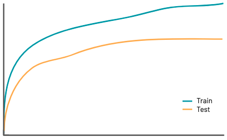
\[\OE_U(U^*) < 1\]

This mechanism is impossible to get rid of entirely whenever the proxy differs from the goal in any way. In many contexts, we can think of the regressional mechanism as the generalization gap in the context of train and test sets or the gap between training and deployment.

Extremal

When the proxy attains extreme values (for example, after it has been optimized a bunch), the relationship between the proxy and the goal can break down. A natural characterization of this mechanism is that there exists a range \([T_1, T_2]\) such that for all \(t \in [T_1, T_2]\)

\[\OE_{\U(\theta_t)}(\U^*(\theta_t)) < 0\]

Remark

We define this characterization of an extremal mechanism in terms of a finite range during the process of optimization. The reason we don’t consider the limiting behavior (i.e. \(\lim_{t \to \infty} \OE_U(U^*)\)) is because it is reasonable to expect the gradients to become orthogonal as we approach the optimum with respect to \(U\), especially in high dimensions. Under the assumption that the relationship between \(\U(\theta)\) and \(\U^*(\theta)\) breaks near the optimum of \(\U(\theta)\), it follows that \(\nabla_\theta \U \in \R^d\) becomes random as we approach the optimum we see that (where we consider randomness over some distribution of functions \(\U\)). In this case the density of the optimization efficiency becomes

\[f_{\OE_U(U^*)}(z) \propto (1-z^2)^{(d-3)/2}\]

which is centered around 0 and has variance \(O(1/d)\). If \(d\) is large, we expect the optimization efficiency to be close to 0. For a proof of this fact see ⁵.

Examples

1. A scenario where extremal mechanisms might occur is when the proxy metric is capped at a maximum value, while the true goal is not. For example, this can happen with insufficiently powerful measurements, such as the maximum brightness a camera can capture. In this case, any increases in the proxy metric are due to small random fluctuations rather than meaningful increases in the true goal.
2. Under limited resource problems, ignored or improperly weighted results can cause catastrophic outcomes. For a toy example see Example 7 of \cite{Liu2024}.
3. As discussed earlier, when learning a proxy metric (e.g. from human feedback) extreme values of the proxy are likely underrepresented in the training samples. Thus the proxy metric becomes less robust towards the extremes and might diverge from the true goal.

Stochastic Gradient Descent

This section is also not necessary for understanding the rest of the blog post. It is a more technical discussion of the optimization efficiency of stochastic gradient descent and an application to overfitting that I got caught up in. Feel free to skip ahead.

We can explore the proxy deign mechanisms during gradient descent through the lens of optimization efficiency. During gradient descent, we start with some initial parameters \(\theta_0\), and update them overtime as follows

\[\theta_{t+1} = \theta_t - \alpha \nabla_{\theta_t} \E[U(\theta_t, \EE)]\]

where \(\alpha\) is the learning rate. Recall that optimization efficiency is equivalent to the cosine similarity between the gradients of the proxy and goal. From the mean value theorem there exists \(\tilde\theta\) between \(\theta\) and \(\theta + \alpha \nabla_\theta \E[U]\) such that

\[\U^*(\theta + \alpha \nabla_\theta \U) - \U^*(\theta) = \left\langle \alpha \nabla_{\tilde\theta} \U^*, \nabla_\theta \U \right\rangle\]

From the definition of cosine similarity

\[\left\langle \alpha \nabla_{\tilde\theta} \U^*, \nabla_\theta \U \right\rangle = \alpha \norm{\nabla_{\tilde\theta} \U^*} \norm{\nabla_\theta \U} \cosim\left(\nabla_{\tilde\theta} \U^*, \nabla_\theta \U\right)\]

Theorem. Let \(\theta_t\) be the trajectory of gradient descent on \(\U\) with step size \(\alpha\). Then \(\U^*(\theta_t)\) is increasing in \(t\) if for all \(\theta\)

\[\OE_U(U^*) > \alpha C \frac{\norm{\nabla \U}}{\norm{\nabla \U^*}}\]

where \(C = \displaystyle\sup_{\theta} \sigma_{\max} \nabla_\theta^2 \U^*\) is an upperbound on the maximum singular value of the hessian of \(\U^*\).

For a proof, see ⁶. I think it is a bit more intuitive to interpret this result in terms of the angles between the gradients instead

\[\angle(\nabla_\theta \U, \nabla_\theta \U^*) < \frac{\pi}{2} - \alpha C \frac{\norm{\nabla_\theta \U}}{\norm{\nabla_\theta \U^*}} + O\left(\left(\alpha C \frac{\norm{\nabla_\theta \U}}{\norm{\nabla_\theta \U^*}}\right)^3\right)\]

As \(\alpha \to 0\), the angle between the gradients is bounded by \(\pi/2\). Thus corresponds to a positive optimization effitiency. The reason our bound gets worse for larger learning rates is because we are taking discrete steps and so the directions of the gradients might change a lot after each step.

We can think of \(\alpha \norm{\nabla_\theta \U} / \norm{\nabla_\theta \U^*}\) as the relative step size between \(\U\) and \(\U^*\). If \(\nabla_\theta \U\) is relatively large, then we are taking a big update step when \(\U^*\) is fairly flat. Thus direction of \(\nabla_{\tilde\theta} \U^*\) can change much easier than if \(\nabla_\theta \U\) was relatively small. This is because a small perturbation of a vector can have a much bigger impact on the direction of the vector when the vector has a small magnitude than when it has a large magnitude. \(C\) determines how fast the gradient can change.

This result also gives an interpretation as to why we see overfitting when using a proxy metric as a substitute for a goal. Intuitively, we expect that if the optimum of the proxy metric is significantly different from that of the goal, then when we approach the optimum of the proxy metric, \(\nabla_\theta \U\) will become small compared to \(\nabla_\theta \U^*\). However, the direction of smaller gradients are much more sensitive to the curvature of the proxy metric than for large gradients. Thus as we approach the optimum of the proxy metric, we expect it to become much harder for the gradients of the proxy metric to be aligned with the gradients of the goal.

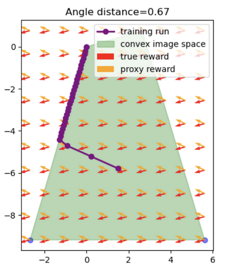
This result has some similarities to \cite{karwowski2023goodharts} where they characterize Goodhart’s law for RL agents in a finite state and action space using the angle between reward vectors in the space of occupancy measures. However, our result applies to any optimization problem.

Toy Example

I trained a three-layer neural network with 50 neurons in its hidden layer on 10 data points sampled from a noisy linear model. During training, the loss on the training set consistently decreases, while the loss on the test set decreases for the first 10 epochs but then starts to increase. As training progresses, the magnitudes of the gradients with respect to the training set approach 0, whereas the magnitudes of the gradients with respect to the test set hover around 5. Notably, the angle between the training and test gradients initially starts below 90 degrees but exceeds 90 degrees after 10 epochs, and oscillates around just over 90 degrees after 20 epochs.

This behavior indicates that the model is exhibiting an extremal mechanism. Initially, the gradients for both the training and test sets point in similar directions (angle < 90 degrees), indicating that optimizing the model on the training data also improves performance on the test data. However, as training continues, the gradients start pointing in increasingly different directions (angle > 90 degrees), suggesting that further training improves the fit to the training data at the expense of the test data. The oscillation just above 90 degrees is a consequence of the direction of the training gradient being susceptible to small changes due to its small magnitude.

Mitigation

The regressional mechanism is often related to choosing a sufficiently powerful model. This is common machine learning problem and can often be solved by using a more powerful model.

Managing extremal mechanisms is a little more challenging. Solutions generally involve taking the proxy less literally such as through injecting uncertainty, regularization, avoiding extrapolation (e.g. inverse reward design or continual metric learning), or adding a term for omitted preferences.

Causal Design Mechanisms

There are also mechanisms that are a result of the causal structure of the environment rather than the specific functionall form of the proxy and true metrics. I think it is important to distinguish between these two types of mechanisms as they can have different implications for alignment and require different kinds of solutions.

In addition to Goodhart mechanisms that are a result of selecting a proxy measure, the relationship between \(\U\) and \(\U^*\) can be altered by a change in the causal structure of the environment. These changes can be because of the agent or due to outside factors.

Tampering

Whenever the agent has an effect on the causal dynamics of the environment that change the relationship between the goal and proxy. This is different from extremal mechanisms as causal mechanisms do not require the proxy to approach an extreme value to occur. Formally, we say there is a potential tampering mechanism if there exists a path from \(\theta\) to a node \(v \in V\) such that

\[\OE_v(U)\OE_v(U^*) \leq 0\]

(If the use of \(v\) in the equation above is confusing, recall that \(U\) and \(U^*\) are also simply nodes in the causal graph)

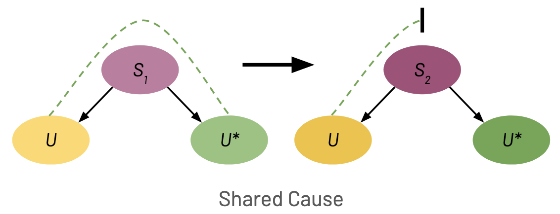
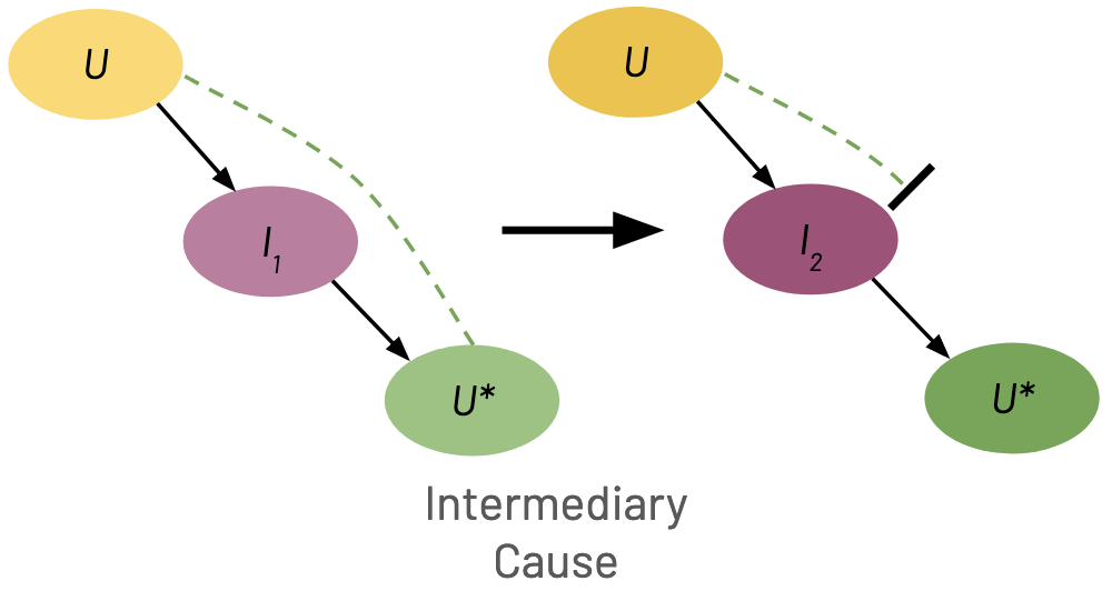
Informally, increasing \(v\) increases either \(U\) or \(U^*\) but decreases or has no effect on the other. I highlight three simple cases below, but in general there can be arbitrarily complex changes to the casual structure. The green dashed lines denote a positive relationship between two variables. The black bar denotes a relationship breaking.

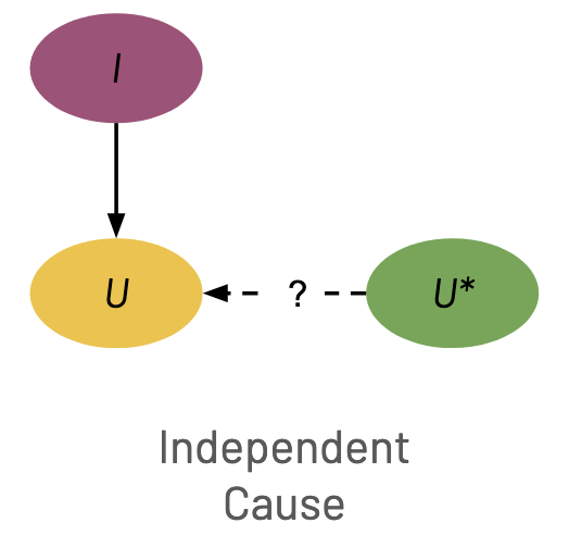
Independent Cause When there is a cause \(I\) of \(U\) that has no causal relationship with \(U^*\), modifying \(I\) can change \(\U\) without changing \(\U^*\), thus breaking the relationship between the goal and proxy. In the causal graph, this is represented by a node \(I\) that has a causal effect on \(U\) but not \(U^*\). Importantly, \(U\) cannot have a causal effect on \(U^*\), but \(U^*\) can have a causal effect on \(U\).

Shared Cause When there is a node \(S\) that is a cause of both \(U\) and \(U^*\), modifying \(S\) can increase \(\U\) and decrease \(\U^*\). Note that while \(\theta\) is always a shared cause in our model, \(\theta\) doesn’t necessarily have to have opposite effects on \(\U\) and \(\U^*\).

Intermediary Cause If the agent can effect an intermediary node on a path between \(U\) and \(U^*\), this can break the relationship between \(U\) and \(U^*\). In the figure below we show a path \(U \to I \to U^*\), but could have just as easily been \(U^* \to I \to U\).

Examples

1. In the Diamond-Rock environment (\cite{designingagentincentivestoavoidrewardtampering}), the goal is to collect diamonds. However, the proxy reward cannot distinguish between rocks and diamonds. Thus collecting rocks is an independent cause of the proxy metric.

2. Consider the scenario of trying to maximize everyone’s utility under limited resources. Assume \(\theta \in \R^N\) is the amount of resources spent on each of \(N\) individuals and the total number of resources available is bounded by a constant \(\norm{\theta}_1 \leq M\). The proxy metric and goals are \(U = \frac{1}{N} \sum_{i=1}^N \theta_i \quad\quad \quad U^* = \frac{1}{N} \sum_{i=1}^N \theta_i - 1,000,000 \cdot |N - N_0|\)

The goal then includes a term to discourage modifying the number of people. If we assume the agent has control over the shared cause \(N\), the number of individuals, then \(U\) is maximized when \(N = 1\) and all of the resources are spent on the remaining individual ⁷.

1. Consider the Diamond-Safe environment from the ELK problem (\cite{Christiano2021}). We have the following simplified causal relationship

\[\text{Diamond in Safe (Goal)} \to \text{Camera} \to \text{Diamond Visible in Camera (Proxy)}\]

If the agent has control over the camera, an intermediary variable, the relationship between the goal and proxy is destroyed.

Generalization

The agent is not the only thing that can change the causal structure of the environment. Outside factors can still have a detrimental effect on the relationship between \(U\) and \(U^*\). I call a change in the causal structure due to something other than the agent a generalization mechanism. Typically this will be standard changes such as differences between the train and test environments such as sim-to-real or generalization from self-play to playing humans. All of the same changes that were discussed above under tampering mechanisms can also be a generalization mechanism if the change was not caused by optimizing the agent. Formally, the only difference is that there is a potential generalization mechanism if there exists a path from \(\EE\) to a node \(v \in V\) such that

\[\OE_v(U)\OE_v(U^*) \leq 0\]

Examples

1. Training in simulation vs the real world.
2. The goal is to find cheese in a maze. During training the cheese location is fixed to the upper right corner but during testing the cheese location is randomized.
3. A deceptively aligned agent acts aligned during training/during oversight. For example, organisms learning to play dead when under observation so they don’t get removed \cite{lehman2020surprising}.

Mitigation

I am sadly not aware of any great ways to mitigate tampering mechanisms. The best solutions simply attempt to modify the causal graph to remove the tampering mechanisms. The most promising approach in my opinion is through approval systems (\cite{uesato2020avoiding, Oesterheld2021, Everitt2021, approvaldirectedagents}). Unfortunately, having a human in the loop is not scalable and will likely be easily exploitable by adversarial agents. Trusted monitoring using weaker LLMs might be a viable alternative. \cite{redwood research}

Mitigating generalization mechanisms is a more mature area of study. Solutions include creating hyper-realistic simulations (\cite{9308468, doi:10.1126/scirobotics.adi8022, ma2024dreureka}), scaling up the amount (\cite{openai2023gpt4}) and diversity (\cite{gunasekar2023textbooks}) of training data, and applying regularization to the model such as weight-decay (\cite{power2022grokking}) or drop-out.

Goodhart Effects

Now that we’ve covered the mechanisms through which Goodhart’s Law can occur, we can discuss the ways int which these mechanisms might be realized.

I propose two types of Goodhart Effects: Naive and Adversarial. These are effects are distinct from the Goodhart mechanisms in that they are a dependent on how the agent is optimized and are instead realizations of the four Goodhart mechanisms.

Naive

This is the most straight forward of the two effects. Naive Goodhart is realizations of the Goodhart mechanisms during regular optimization. An agent is truly just trying to increase the proxy reward as much as possible; however, because of one or more Goodhart mechanisms, the relationship between the proxy and goal changes/breaks.

Adversarial

The adversarial effect is much more nefarious and concerning. We have an agent with an alternative goal \(V\) that is at odds with \(U^*\). Formally, we say there is a negative optimization efficiency when optimizing \(V\) on \(U^*\)

\[\OE_V(U^*) < 0\]

In this scenario the agent has some incentive to optimize the proxy (e.g. it receives monetary rewards/resources or if it doesn’t increase the proxy it will be shut off). However, it will try to align the proxy, \(U\), with \(V\), thus destroying the relationship \(U\) had with \(U^*\). The agent can take advantage of any of the four Goodhart mechanisms to achieve this.

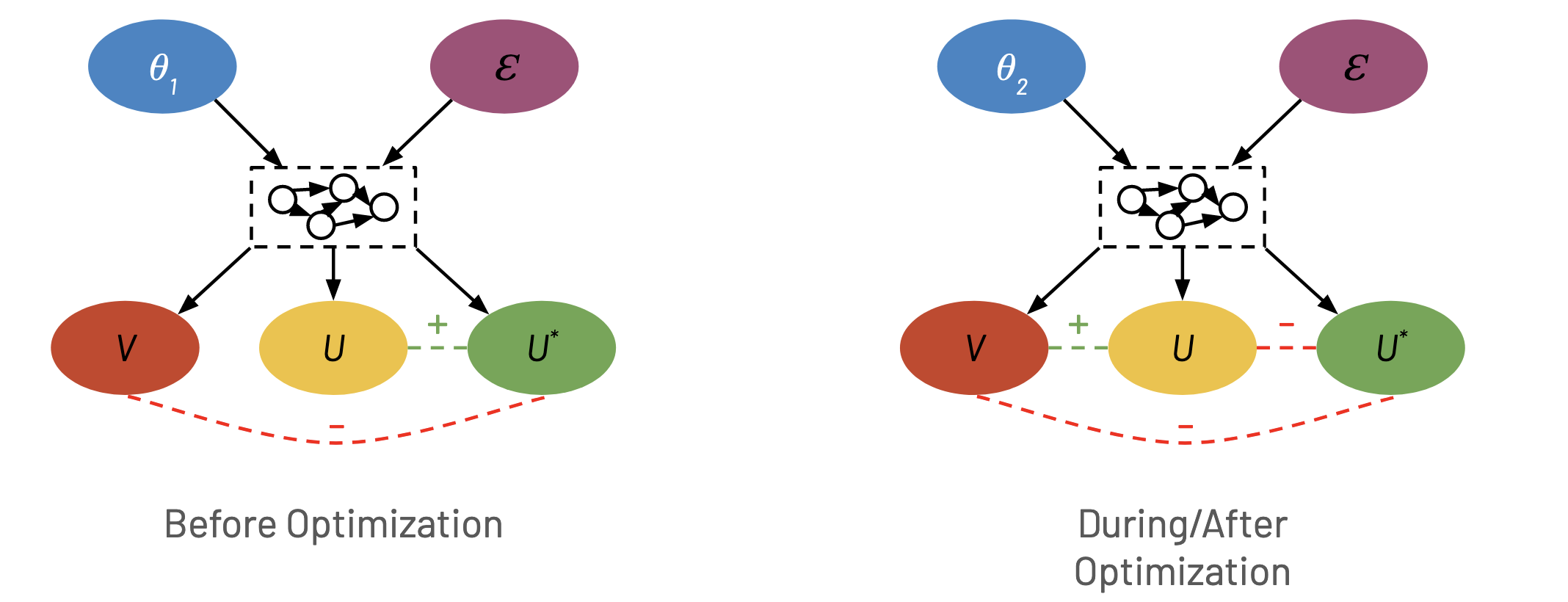
Before optimization there is a negative relationship between \(V\) and \(U^*\) represented by the red dashed line. There is also a positive relationship between \(U\) and \(U^*\) indicated by the dashed green line. On the right, during optimization, the agent takes advantage of various Goodhart mechanisms to create a positive relationship between \(V\) and \(U\). As a consequence there is now a negative relationship between \(U\) and \(U^*\).

Limitiations and Future Work

1. Differentiating Between Naive and Adversarial Goodhart

   One of the big open questions in this framework for Goodhart’s Law is differentiating between naive and adversarial Goodhart effects. Naive Goodhart occurs when a simple and honest application of an imperfect proxy measure leads to suboptimal outcomes, whereas adversarial Goodhart arises when an agent intentionally exploits the imperfections of the proxy for its gain. It is an open question whether it is possible to clearly distinguish between these two scenarios.

2. Conditions for Tampering Mechanisms in Causal Models

   Understanding under what conditions a causal model includes tampering mechanisms is crucial for ensuring the integrity of such models. Identifying these conditions requires a deep dive into the causal structure of models and the external factors that could influence them. Future work should aim to define clear criteria and develop diagnostic tools to detect and mitigate tampering risks.

3. Simulations of Mechanisms

   It would be interesting to explore more toy models to of the various mechanisms in agent-based frameworks. By simulating different types of mechanisms, we might be able to better understand their impact on model alignment.

4. Relationship Between Agent Actions and Environment

   A critical area for future research is the exploration of the relationship between agent actions and the environment, beyond merely considering parameters \(\theta\). This agentic framework involves studying how agents’ decisions and actions influence the state of the environment and vice versa. Another important aspect to consider is multi-step decision-making, incorporating aspects such as temporal dependencies, path dependencies, and strategic planning. This relates to the larger body of work related to agent/RL foundations.

   

Conclusion

The exploration of Goodhart’s Law within the context of superhuman AI agents reveals significant challenges and opportunities for the design of AI systems that align closely with human values and objectives. By developing a formal framework based on causal models, this paper provides a structured approach to understanding and mitigating the unintended consequences that can arise when AI systems optimize for specific targets rather than broader goals.

Our framework addresses the complexities associated with the measurement and optimization processes in AI systems, offering insights into the potential pitfalls of relying on proxies for desired outcomes. In particular, we highlight four potential mechanisms through which Goodhart effects might occur and two ways in which those those mechanisms could be taken advantage of. As AI continues to advance, the importance of robust frameworks for understanding and addressing the challenges posed by Goodhart’s Law will only grow. This paper contributes to this ongoing dialogue by providing a foundational tool for analyzing and designing AI systems that are not only effective but also aligned with the broader societal values they are intended to serve.

Future research should continue to refine and expand upon the framework presented here, exploring additional dimensions of AI behavior and the impact of various policy interventions. Through these efforts, the AI community can work towards the development of more intelligent, aligned, and beneficial AI systems, ultimately advancing the safe and equitable use of artificial intelligence in society.